Deconvolution.jl

Introduction

Deconvolution.jl provides a set of functions to deconvolve digital signals, like images or time series. This is written in Julia, a modern high-level, high-performance dynamic programming language designed for technical computing.

Installation

The latest version of Deconvolution.jl is available for Julia 1.0 and later versions, and can be installed with Julia built-in package manager. In a Julia session, after entering the package manager mode with ], run the command

pkg> add Deconvolution

Older versions are also available for Julia 0.4-0.7.

Usage

Currently Deconvolution.jl provides only two methods, but others will hopefully come in the future.

`wiener` function

The Wiener deconvolution attempts at reducing the noise in a digital signal by suppressing frequencies with low signal-to-noise ratio. The signal is assumed to be degraded by additive noise and a shift-invariant blurring function.

Theoretically, the Wiener deconvolution method requires the knowledge of the original signal, the blurring function, and the noise. However, these conditions are difficult to met (and, of course, if you know the original signal you do not need to perform a deconvolution in order to recover the signal itself), but a strength of the Wiener deconvolution is that it works in the frequency domain, so you only need to know with good precision the power spectra of the signal and the noise. In addition, most signals of the same class have fairly similar power spectra and the Wiener filter is insensitive to small variations in the original signal power spectrum. For these reasons, it is possible to estimate the original signal power spectrum using a representative of the class of signals being filtered.

For a short review of the Wiener deconvolution method see http://www.dmf.unisalento.it/~giordano/allow_listing/wiener.pdf and references therein.

The wiener function can be used to apply the Wiener deconvolution method to a digital signal. The arguments are:

input: the digital signal
signal: the original signal (or a signal with a likely similar power spectrum)
noise: the noise of the signal (or a noise with a likely similar power spectrum)
blurring (optional argument): the blurring kernel

All arguments must be arrays, all with the same size, and all of them in the time/space domain (they will be converted to the frequency domain internally using fft function). Argument noise can be also a real number, in which case a constant noise with that value will be assumed (this is a good approximation in the case of white noise).

`lucy` function

The Richardson-Lucy deconvolution is an iterative method based on Bayesian inference for restoration of signal that is convolved with a point spread function.

The lucy function can be used to apply the Richardson-Lucy deconvolution method to a digital signal. The arguments are:

observed: the digital signal
psf: the point spread function
iterations (optional argument): the number of iterations

First two arguments must be arrays, all with the same size, and all of them in the time/space domain (they will be converted to the frequency domain internally using fft function). Argument iterations is an integer number. The more iterations is specified the better result should be if the solution converges and it is going to converge if PSF is estimated well.

Examples

Wiener deconvolution

Noisy time series

This is an example of application of the Wiener deconvolution to a time series.

We first construct the noisy signal:

using LombScargle, Deconvolution, Plots, Statistics
t = range(0, stop=10, length=1000) # observation times
x = sinpi.(t) .* cos.(5 .* t) - 1.5 .* cospi.(t) .* sin.(2 .* t) # the original signal
n = rand(length(x)) # noise to be added
y = x .+ 3 .* (n .- mean(n)) # observed noisy signal

In order to perform the Wiener deconvolution, we need a signal that has a power spectrum similar to that of the original signal. We can use the Lomb–Scargle periodogram to find out the dominant frequencies in the observed signal, as implemented in the the Julia package LombScargle.jl.

# Lomb-Scargle periodogram
p = lombscargle(t, y, maximum_frequency=2, samples_per_peak=10)
plot(freqpower(p)...)

After plotting the periodogram you notice that it has three peaks, one in each of the following intervals: $[0, 0.5]$, $[0.5, 1]$, $[1, 1.5]$. Use the LombScargle.model function to create the best-fitting Lomb–Scargle model at the three best frequencies, that can be found with the findmaxfreq function (see the manual at https://juliaastro.github.io/LombScargle.jl/stable/ for more details):

m1 = LombScargle.model(t, y, findmaxfreq(p, [0, 0.5])[1]) # first model
m2 = LombScargle.model(t, y, findmaxfreq(p, [0.5, 1])[1]) # second model
m3 = LombScargle.model(t, y, findmaxfreq(p, [1, 1.5])[1]) # third model

Once you have these three frequencies, you can deconvolve y by feeding wiener with a simple signal that is the sum of these three models:

signal = m1 + m2 + m3 # signal for `wiener`
noise = rand(length(y)) # noise for `wiener`
polished = wiener(y, signal, noise)
plot(t, x, size=(900, 600), label="Original signal", linewidth=2)
plot!(t, y, label="Observed signal")
savefig("time-series-observed.png")
plot(t, x, size=(900, 600), label="Original signal", linewidth=2)
plot!(t, polished, label="Recovered with Wiener")
plot!(t, signal, label="Lomb–Scargle model")
savefig("time-series-recovered.png")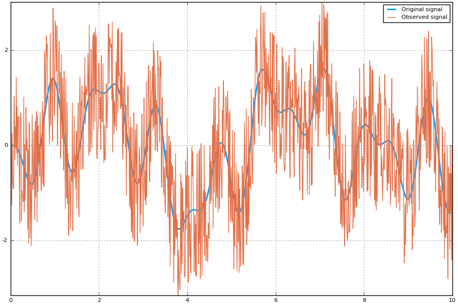

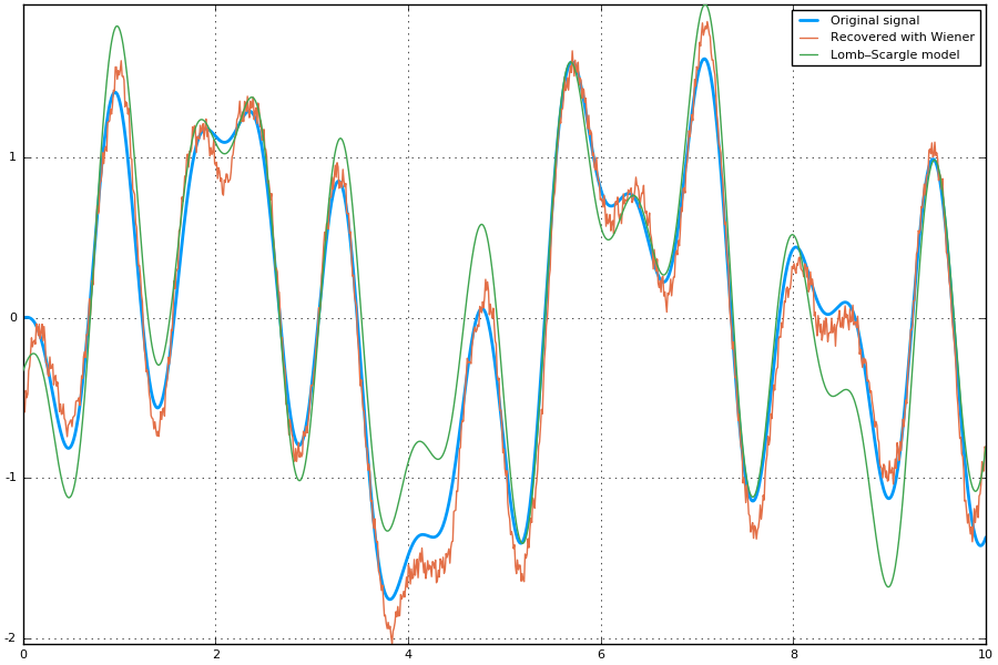
Note that the signal recovered with the Wiener deconvolution is generally a good improvement with respect to the best-fitting Lomb–Scargle model obtained using a few frequencies.

With real-world data the Lomb–Scargle periodogram may not work as good as in this toy-example, but we showed a possible strategy to create a suitable signal to use with wiener function.

Blurred noisy time series

Additionally to noise, also a blurring kernel can applied to the image. First we define the blurring kernel as a Gaussian kernel. Using ifftshift we move the center to index position 1 which is required for the Wiener deconvolution algorithm.

# Gaussian blurring kernel
kernel = exp.( -10 .* (t .- 5) .^ 2)
kernel ./= sum(kernel) # normalize kernel to sum of 1
kernel = ifftshift(kernel) # move center to index pos 1

The blurring can be applied simply in Fourier space. After the blurring we add the noise.

y_blurred = real(ifft(fft(kernel) .* fft(x))) + noise

The deblurred image can be obtained with the following call.

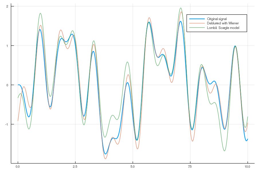
deblurred = wiener(y_blurred, signal, noise, kernel)

Additionally to the noise array we also pass kernel to wiener.

plot(t, x, size=(900, 600), label="Original signal", linewidth=2)
plot!(t, deblurred, label="Deblurred with Wiener")
savefig("time-series-deblurred.png")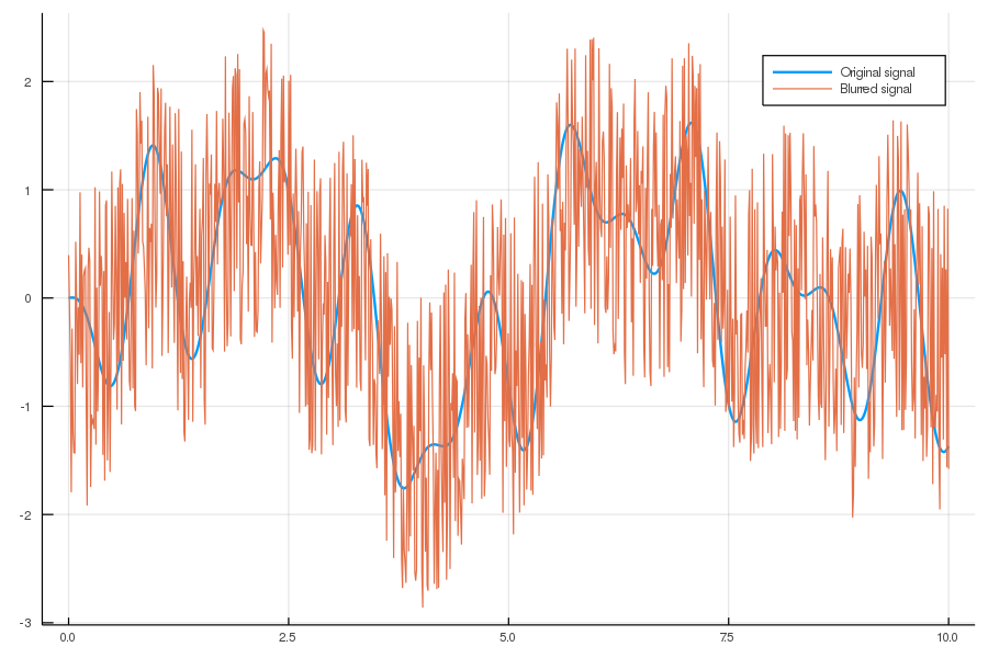

Blurred image

Here is an example of use of wiener function to perform the Wiener deconvolution of an image, degraded with a blurring function and an additive noise.

using Images, TestImages, Deconvolution, ImageView

# Open the test image
img = float(data(testimage("cameraman")))'
# Create the blurring kernel in frequency domain
x = hcat(ntuple(x -> collect((1:512) - 257), 512)...)
k = 0.001
blurring_ft = exp.(-k .* (x .^ 2 .+ x' .^ 2) .^ (5//6))
# Create additive noise
noise = rand(size(img))
# Fourier transform of the blurred image, with additive noise
blurred_img_ft = fftshift(blurring_ft) .* fft(img) + fft(noise)
# Get the blurred image from its Fourier transform
blurred_img = real(ifft(blurred_img_ft))
# Get the blurring kernel in the space domain
blurring = ifft(fftshift(blurring_ft))
# Polish the image with Deconvolution deconvolution
polished = wiener(blurred_img, img, noise, blurring)

# Wiener deconvolution works also when you don't have the real image and noise,
# that is the most common and useful case.  This happens because the Wiener
# filter only cares about the power spectrum of the signal and the noise, so you
# don't need to have the exact signal and noise but something with a similar
# power spectrum.
img2 = float(data(testimage("livingroom"))) # Load another image
noise2 = rand(size(img)) # Create another additive noise
# Polish the image with Deconvolution deconvolution
polished2 = wiener(blurred_img, img2, noise2, blurring)

# Wiener also works using a real number instead of a noise array
polished3 = wiener(blurred_img, img2, 1000, blurring)
polished4 = wiener(blurred_img, img2, 10000, blurring)


# Compare...
view(img) # ...the original image
view(blurred_img) # ...the blurred image
view(polished) # ...the polished image
view(polished2) # ...the second polished image
view(polished3) # ...the third polished image
view(polished4) # ...the fourth polished image

Original image	Blurred image

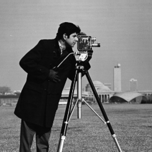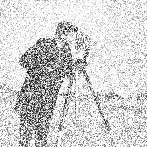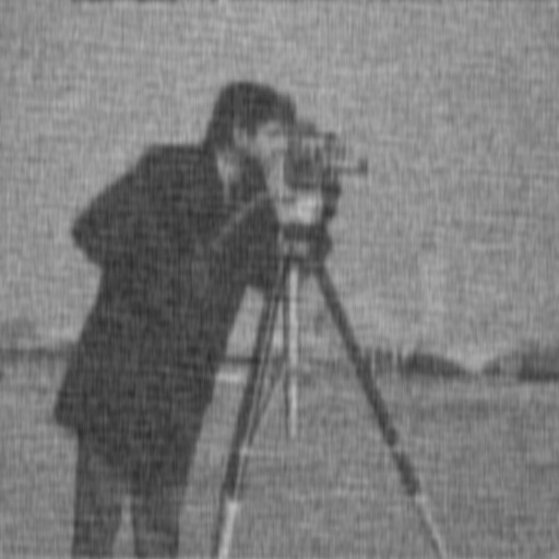
Image restored with exact power spectrum and noise	Image restored with imperfect reference noise and spectrum

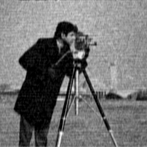Image restored with imperfect spectrum and constant noise	Image restored with imperfect spectrum and constant noise

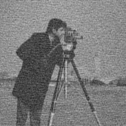Without knowing the noise array exactly the contrast drops significantly. Some postprocessing of the contrast can enhance the quality further.

Richardson-Lucy deconvolution

Blurred image

Here is an example of use of lucy function to perform the Richardson-Lucy deconvolution of an image convolved with point spread function that models lens aberration.

    using Images, TestImages, Deconvolution, FFTW, ZernikePolynomials, ImageView

    img = channelview(testimage("cameraman"))

    # model of lens aberration
    blurring = evaluateZernike(LinRange(-16,16,512), [12, 4, 0], [1.0, -1.0, 2.0], index=:OSA)
    blurring = fftshift(blurring)
    blurring = blurring ./ sum(blurring)

    blurred_img = fft(img) .* fft(blurring) |> ifft |> real

    @time restored_img_200 = lucy(blurred_img, blurring, iterations=200)
    @time restored_img_2000 = lucy(blurred_img, blurring, iterations=2000)

    imshow(img)
    imshow(blurred_img)
    imshow(restored_img_200)
    imshow(restored_img_2000)

Original image	Blurred image

Result of 200 `lucy` iterations	Result of 2000 `lucy` iterations

Development

The package is developed at https://github.com/JuliaDSP/Deconvolution.jl. There you can submit bug reports, propose new deconvolution methods with pull requests, and make suggestions. If you would like to take over maintainership of the package in order to further improve it, please open an issue.

History

The ChangeLog of the package is available in NEWS.md file in top directory.

License

The Deconvolution.jl package is licensed under the MIT "Expat" License. The original author is Mosè Giordano.